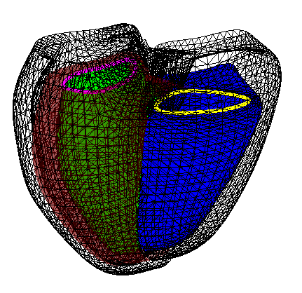
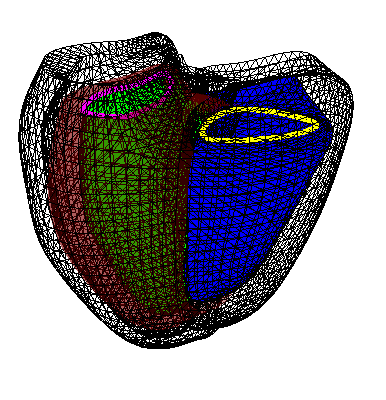
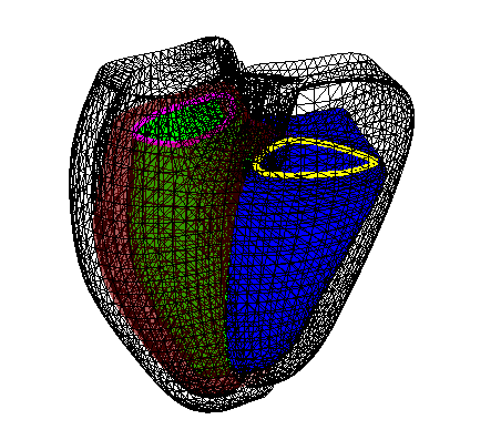
These are PCA modes of variations from biventricular shapes derived from ~5,000 UK Biobank cardiac MRI exams. You can read more information about this study from [Mauger et al., JCMR 2019]. Each figure contains two biventricular models from End-Diastole (wireframe without surface color) and End-Systole (coloured surface: green = left ventricle, blue = right ventricle, red = myocardium, pink contour = mitral valve, and yellow contour = tricuspid valve).

Download
We provide two Principal Component Analysis (PCA) atlases:
UKBRVLV.h5contains PCA atlas derived from 630 healthy reference subjects from the UK Biobank Study (see [Petersen et al., 2017]).UKBRVLV_ALL.h5contains PCA atlas derived from all 4,329 subjects from the UK Biobank Study.
Only the first 200 PCA components are shared. The PCA structure is defined as follows:
/COEFF: N x 200 matrix of the first 200 principal components, where N is the number of sample points/LATENT: 200 elements vector of the eigenvalues,/EXPLAINED: 200 elements vector that show the percentage of the total variance explained by each principal component,/MU: N elements vector that defines the mean shape of the biventricular model.
The file is saved in HDF5 format. Below is an example on how to read and plot the first principal mode.
from mpl_toolkits.mplot3d import Axes3D
import matplotlib.pyplot as plt
import h5py as h5
import numpy as np

# read H5 file
pc = h5.File('UKBRVLV.h5', 'r')

# note that H5PY matrices in python are transposed

# generate the first principal mode
# with 1.5 times the standard deviation
S = np.transpose(pc['MU']) + (1.5 * np.sqrt(pc['LATENT'][0,0]) * pc['COEFF'][0,:])

# get ED & ES points, & convert to 3 columns matrix [x, y, z]
N = S.shape[1] // 2
ed = np.reshape(S[0,:N], (-1,3))
es = np.reshape(S[0,N:], (-1,3))

# plot ED points in blue
# plot ES points in red
fig = plt.figure()
ax = fig.add_subplot(111, projection='3d')
ax.scatter(ed[:,0], ed[:,1], ed[:,2], color='dodgerblue', marker='.')
ax.scatter(es[:,0], es[:,1], es[:,2], color='firebrick', marker='.')
% read the principal components
pc = h5read('UKBRVLV.h5', '/COEFF');

% read the eigenvalues
ev = h5read('UKBRVLV.h5', '/LATENT');

% read the mean shape
mu = h5read('UKBRVLV.h5', '/MU');

% generate the first principal mode
% with 1.5 times the standard deviation
S = mu + (1.5 .* sqrt(ev(1)) .* pc(:,1)');

% get ED & ES points, & convert to 3 columns matrix [x, y, z]
N = length(S);
ed = reshape(S(1:N/2), 3, [])';
es = reshape(S((N/2+1):end), 3, [])';

% plot ED points in blue
% plot ES points in red
figure('Color', 'w');
plot3(ed(:,1), ed(:,2), ed(:,3), 'b.');
hold on;
plot3(es(:,1), es(:,2), es(:,3), 'r.');
axis vis3d
axis equal
library(h5)
library(rgl)

# read H5 file
f = h5file("UKBRVLV.h5")

# read the principal components
pc = f["/COEFF"]

# read the eigenvalues
ev = f["/LATENT"]

# read the mean shape
mu = f["/MU"]

# generate the first principal mode
# with 1.5 times the standard deviation
S = t(mu[]) + (1.5 * as.numeric(sqrt(ev[1,1])) * pc[1,])

# get ED & ES points, & convert to 3 columns matrix [x, y, z]
N = length(S);
ed = matrix(S[1, 1:(N/2)], ncol=3, byrow=TRUE)
es = matrix(S[1, (N/2+1):N], ncol=3, byrow=TRUE)

# plot ED points in blue
# plot ES points in red
plot3d(ed[,1],ed[,2],ed[,3], col="dodgerblue3", size=1)
plot3d(es[,1],es[,2],es[,3], col="firebrick3", size=1, add=TRUE)